Real-time deformation of solids, Part 1
 In the last few years, an important hardware gap has been filled by the video game industry: the GPU have replaced the
CPU and software emulation.
Although physics simulation has been extensively studied since the beginning of the computer age, this kind of simulation paradoxically remains little explored by video games.
In the last few years, an important hardware gap has been filled by the video game industry: the GPU have replaced the
CPU and software emulation.
Although physics simulation has been extensively studied since the beginning of the computer age, this kind of simulation paradoxically remains little explored by video games.
Let us take the case of physics simulation. Before the birth of the computer age, physicians had come up with many analytical equations for various physical problems. But unfortunately, these equations were focusing on simple cases. When computer started being used, analytical equations finally allowed finding approximate solutions; it was the beginning of the numerical computation.
Numerical methods enable engineers to expand their abilities to solve practical design problems. They now treat real shapes as distinct from the somewhat limited variety of shapes from simple analytic solution. Similarly, they do not need to force a complex loading system to fit a more regular load configuration in order to conform to a purely academic situation. Numerical analysis thus provides a tool with which the engineer may feel free to look for the solution of practical problems.
Real-time vs. Generic solutions
Numerical and analytical techniques cannot be easily adapted to video games because:
- On one side, interactive virtual worlds must simulate a large variety of physical problems, each problem being different. For example, the player throws a stone in a closed room and the stone moves according to the starting velocity, the geometry of the room and player's orientation and position. Analytical solution of the stone trajectory differs each time, so the only choice consists in computing the displacement step by step. Consequently, having a fully analytical formula of a physical phenomenon is very difficult to elaborate.
- On the other side, numerical computation, often iterative, is rarely possible in real-time. The computation takes several minutes, sometimes hours or days to solve standard engineering problems. It is then difficult to achieve simulation in real-time without simplification beforehand.
Realistic vs. Real solutions
The last aspect of physics simulation is the duality between the realistic appearance and the real. A real solution is an correct solution. In such case we admit that a solution is correct when the difference between the theory and the solution is negligible in comparison with the dimension of the physical problem. On the other hand, a realistic solution can seem to be physically correct. It is a relative notion which depends on the observer. If the simulated trajectory of a stone bouncing off the wall differs from the reality by several centimeters, the observer of this simulation may still admit that the trajectory was real.
That is why particle systems are often used in video games. In this case, the simulation is not physically correct but is realistic. Simplifying the reality may not be a problem if the results look realistic enough.
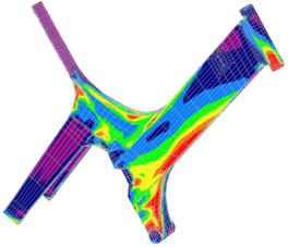
Deformation of solids in real-time
I have opted to concentrate on elements that have not been really studied by the game industry. So I have selected the deformation of solids such as steel or concrete structures. Deformations of solids could occur in many occasions during a game: a car crashes into a wall, or a player fires a rocket into a structure.
Preliminary definitions
The basic structure of the matter is characterized by non-uniformity and discontinuity attributable to its various subdivisions: molecules, atoms and subatomic particles. The concern in this document is to replace the actual system of particles with a continuous distribution of matter. There is the clear implication in such an approach that any small volumes which could be considered here are enough to contain a lot of particles. Random fluctuations in the properties of the material are not considered to be important.
The studied system is a solid, which is sometimes referred to by the name of body. Some of the main abilities of a solid are:
- to maintain its shape without need of a container.
- to resist continuous shear and tension.
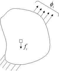
In contrast with rigid body statics and dynamics, which treat the external behavior of bodies, the mechanics of solids are concerned with the relationship of external effects (i.e. forces and moments) to internal stresses and strains. External forces actions on a body may be classified as surface forces and body forces. A surface force is of the concentrated type when it acts at a point; a surface force may also be distributed uniformly or non-uniformly over a finite area. Body forces act on volumetric elements rather than surfaces and are attributable to fields such as gravity and magnetism.
All the units follow the international standard (IS). The right-handed system is used by default.
| Data | Dimension | Symbol |
| Length | Meter | m |
| Force | Newton | N |
| Pressure | Pascal | Pa |
| Masse | Kilogram | kg |
The Finite Element Method
In this article, I will explain how to build a simulation which:
- is real-time.
- obtains realistic results
- handles a large variety of shapes for the solid.
- applies various boundary conditions.
The only tolerated hypothesis is that the deformations always occur in the elastic domain, i.e. there is a linear relation between the applied forces and the displacements.
To succeed in this task, classic analytical methods used in the mechanics of solids are limited. Strength of Materials has resolved some problems but they are too specific. Navier relations for plates and shells are also not generic enough. In conclusion, analytical methods seem to be less adapted than numerical methods. Nowadays, the most powerful method to resolve physical problems is a numerical method called the Finite Element Method (FEM).
The Finite Element Method originates in the 1950's. With the widespread use of the computers, this method has since gained considerable favor compared to other numerical approaches. This method allows to predict stress and strain in an engineering structure with unprecedented ease and precision. In this article, we only discuss about continuum mechanics and its applications within the FEM.
The general procedure of the finite element and conventional structural matrix methods are similar. Consequently, the later method will be first presented. For more information, FEMUR (Finite Element Method Universal Resources) provides a wealth of resources. I also recommend to read The Finite Element Method in Engineering Science by Zienkiewicz, FEM/BEM Notes by Hunter and Pullan, as well as Accurate Real Time Deformable Object by James and Pai.
Structural Matrix Method
This method allows to calculate the displacement and the stress in a structure usually made of beams. The structure is idealized as an assembly of structural members connected to one another at joints or nodes at which the resultants of the applied forces are assumed to be concentrated.
Employing the mechanics of solids or the elasticity approach, the stiffness properties of each element can be ascertained. Equilibrium and compatibility considered at each node lead to a set of algebraic equations, in which the unknowns may be nodal displacements, internal nodal forces, or both, depending on the specific method used.
In the displacement or so-called direct stiffness method, the set of algebraic equations involves the nodal displacements. In the force method, the equations are expressed in terms of unknown internal nodal forces. A mixed method is also used, in which the equations contain both nodal displacements and internal forces.
Case of One Spring
One of the simplest cases from the structural matrix method is to idealize each member of the structure by a spring. The stability of an
elastic spring is characterized by its constant of rigidity  . This constant is used to calculate the return force
  .
.
The relation linking displacement and force is  .
.  is the relative length variation of the spring. When two axial forces are applied to the spring, the stability commands that:

 are respectively the forces and the displacements for each node.
A matrix relation could replace these equations. The matrix, which links the force vector and the displacement vector, is called the stiffness matrix of the spring:
Case of Three Springs
We could assemble several elements modeled with springs to construct more complex structures.
After assembling the three stiffness matrices of the element, a linear relation that links the forces and the displacement is found:

S is the section of the element. E is the Young modulus of the material.
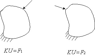
Notice that the problem has 6 unknowns (3 nodes free along the x and the y axes), which are organized in the vector. To resolve the problem, we apply boundary conditions: the nodes 1 and 3 are fixed in the three directions. After resolving the displacements of the node 2, the reaction forces, which are applied on the nodes 1 and 3, are found. The fundamental relation that must be remembered is the matrix relation . As we are going to see, with the finite element method, theses relations could be computed for any continuous body and so not only for structures.
The structural approach is comparable in some ways with some computing methods, famous in the field of the video games. The most interesting articles are 2D Surface Deformation by Max I. Fomitchev or Real-Time Cloth Animation by Jeff Lander. Another interesting application includes a game using the structural approach to calculate stress in bridges.
Principles of the FEM
In contrast to the structural matrix method, the solid continuum in the finite element method is divided into a finite number of elements, connected not only on their nodes, but along the hypothetical inter-element boundary as well. In addition to nodal compatibility and equilibrium, compatibility must also be met along the boundaries between the elements. Therefore the element stiffness can only be approximately determined.
As in the structural analyze, there are several approaches for the FEM. In this article, we treat only the commonly employed finite element displacement approach.
Theory
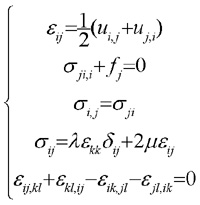
Let us take a stress analysis problem for a body under certain loading conditions.
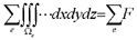
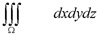
The normal analytical procedure would involve taking an extremely small box element of dimensions (dx, dy, dz) each tending to zero and then writing down the equations of equilibrium and compatibility for this element.
Then we would try to obtain a solution for the stress distribution in the body under the specified boundary conditions using the integration techniques over the entire body. The drawback of this method is that for complicated bodies it will be very difficult and sometimes impossible to carry out the integration procedure over the entire body.
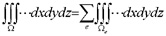
The solution to such problems can be obtained very effectively and to a high degree of accuracy using the Finite Element Method. Instead of assuming a displacement field for the entire body, we divide the body into smaller elements and assume a displacement field for these individual elements. The original body or structure is then considered as an assemblage of these elements. Once again, these elements are connected to each other at joints called nodes or nodal points to form the entire structure. These individual elements are now analyzed. Instead of carrying out integration over the entire body consisting of infinite number of elements of infinitesimally small dimensions, we carry out summation over the body consisting of finite number of elements of finite dimensions. By this iterative approach, the method can be effectively implemented in a computer program.
The equations of equilibrium for the entire structure or body are then obtained by combining the equilibrium equation of each element so that the continuity is ensured at each node. The necessary boundary conditions are then imposed and the equations of equilibrium are solved to obtain the required variables such as stress, strain, temperature, distribution or velocity flow depending on the application.
 |
|
| Boundary Conditions | |
 |
|
| Algebraic equations | |
 |
We must also realize that FEM is a numerical technique and the answers obtained are not the exact solutions but only approximate. However by using appropriate procedures and proper computing techniques, we can obtain an extremely high degree of accuracy which is very much acceptable in practice. Notice that the "acceptable" term is used for engineering problems. In the video games field, after using acceptable procedures, the result can be considered physically correct.
The structural matrix method is finally similar to the FEM. Actually the divided structures of beams are replaced by continuum solids.
| Physical system | ||
| Equations with partial derivatives | ||
| Integral formulation | ||
| Analytical method | FEM | |
 |
 |
|
| ? Difficulty to carry out the integration procedure |
Systems of algebraic equations | |
| Approximate Solution |
Stiffness matrix
The stiffness matrix of a three-springs element has been formulated previously. The finite element method can also work with more complicated elements of two or three dimensions.
In this article, the only studied element is a cube made of eight nodes with three degrees of freedom by nodes. In fact, each node can move along the x, y and z axes. In the previously example with the one spring, the nodes located at each extremities of the element were moving only along the axis of the spring.
Consequently, the dimension of the stiffness matrix of this element is 24 by 24:
The matrix depends only on the material properties and dimensions of the cube. The analytical form has been calculated with Maple.
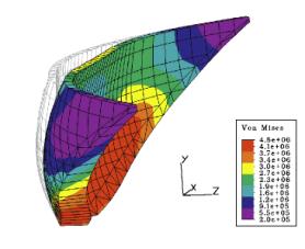
Common applications of the Finite Element Method
FEM has a wide range of applications such as stress analysis, heat transfer, fluid flow, or torsion analysis. In this article, I will demonstrate that it is possible to adapt these industrial cases for video games.


FEM implementation for real-time scenarii
The common steps for a calculation based on the FEM follows:
| Pre-processing | Property of the material, geometric shape of the body |
| Meshing (the division of the body is done into finite elements) | |
| Computation of each stiffness matrix | |
Construction of the global matrix  |
|
| Solution | Boundary conditions (degree of freedom, loading) |
| Application of the boundary conditions | |
| Resolution of the system |
|
| Post-Processing | Display results |
| Data entry | |
| Computation step |
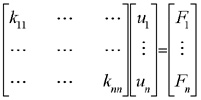
In order to find the displacements of nodes, we must resolve the linear system . depends only on the geometry, the characteristics of the material, the number and the shape of the finite elements. Consequently, and it is the most important, the matrix does not depend on the applied forces.
To resolve the matrix system, finite element applications use Gauss elimination, substitution or Newton-Raphson methods. These methods
manipulate the second member of the equation (i.e. the force vector ), and of course these methods are the fastest. For example, the computation time to resolve a system within 10 000 degrees of freedom is about one minute. Of course it is not in real-time. Therefore the system needs to be resolved independently of the force vector.
The solution is to compute the inverse of the matrix. But everyone knows that the inversion of matrix is a slow computation, but does it matter? If the solution doesn't depend on the force vector, the system can be resolved before the beginning of the application. For example, the inverse of the matrix is stored in a file and loaded during the initialization of the application (typically during the loading of a game level). The drawback of this method is that the boundary conditions are fixed and could not change. In fact, to inverse the matrix, simplification is done according to the boundary conditions.
| Construction of the level | Loading of the level |  Execution of the level - Needs to be in real-time Execution of the level - Needs to be in real-time |
|
 |
 |
||
| Classic method | Construction of the global matrix Application of the boundary conditions |
Loading of the global matrix |
Application of the boundary conditions Resolution of the system with the Gauss method |
| Adapted method | Construction of the global matrix Application of the boundary conditions Inversion of the global matrix |
Loading of the inversed global matrix |
Matrix multiplication |
Hyperion Project
The Hyperion project provides an implementation of the technique described in this article. The sources are licensed under LGPL (Lesser General Public License) and can be found on the web site of the project.
 The Hyperion project is built on top of a component-based architecture.
During the year 1999, I worked for an industrial software company specialised in real-time and embedded systems. There, I developed a mechanism similar to COM and adapted for the Unix, Windows, and VxWorks operating systems. This mechanism was re-adapted for the needs of the project.
The Hyperion project is built on top of a component-based architecture.
During the year 1999, I worked for an industrial software company specialised in real-time and embedded systems. There, I developed a mechanism similar to COM and adapted for the Unix, Windows, and VxWorks operating systems. This mechanism was re-adapted for the needs of the project.
Library of specialized components
 With the help of this architecture, the applications could be not only object-oriented but also could be component-oriented.
In order to test on a large scale the new developed architecture, I created the first components specialised in the physical simulation in real-time. The long-term prevision is to set a coherent library of components in the same way as DirectX is specialised in multimedia.
With the help of this architecture, the applications could be not only object-oriented but also could be component-oriented.
In order to test on a large scale the new developed architecture, I created the first components specialised in the physical simulation in real-time. The long-term prevision is to set a coherent library of components in the same way as DirectX is specialised in multimedia.
 The most important is the set of components called the Ephydryne components. The Ephydryne components compute the deformation of solids and so realize the specifications explained in the previous part. The Ephydryne package defines a set of interface and implements the necessary components to make all the necessary computing steps. To prove the capabilities of the Ephydryne components and the viability of the chosen solutions, two client applications have been developed, HypDev and HypVisual.
Two steps and two tools
 It is a client application that uses the Ephydryne components. The goal of HypDev is to calculate the linear relations between the forces
applied on the rigid bodies and the deformations. According to the method presented in this article, the linear relation is computed
during the development of the level. Again the linear relation is consequently loaded during the execution of the level. So an important
part of the computation is not done during the game (step which is in real-time).
It is a client application that uses the Ephydryne components. The goal of HypDev is to calculate the linear relations between the forces
applied on the rigid bodies and the deformations. According to the method presented in this article, the linear relation is computed
during the development of the level. Again the linear relation is consequently loaded during the execution of the level. So an important
part of the computation is not done during the game (step which is in real-time).
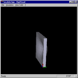
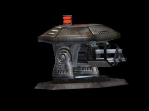
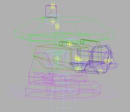
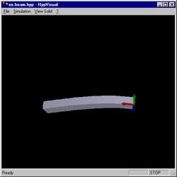
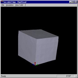
 The step which is in real time is studied with the application called HypVisual. This application loads the file generated by HypDev, displays the body and manages the simulation.
|
|
|
The second part of this article will go though the use of the Ephydryne components and will provide more technical details about the implementation.
Note: This article was originally published on Gamedev in August 2001. It has been updated and slightly reorganized in this present version.