Rolling median with Azure Data Lake Analytics
Azure Data Lake Analytics (DLA in short) provides a rich set of analytics functions to compute an aggregate value based on a group of rows. The typical example is with the rolling average over a specific window. Below is an example where the window is centered and of size 11 (5 preceding, the current row, and 5 following). The grouping is made over the site field.
   SELECT
        AVG(value) OVER(PARTITION BY site ORDER BY timestamp ROWS BETWEEN 5 PRECEDING AND 5 FOLLOWING) AS rolling_avg
    FROM @Data;
However, the median function does not support the ROWS option. It is not possible therefore to run rolling median straight out of the box with DLA.
PERCENTILE_DISC(0.5) WITHIN GROUP(ORDER BY value) OVER(PARTITION BY site, timestamp ROWS BETWEEN 5 PRECEDING AND 5 FOLLOWING) AS rolling_median // will generate an errorThe aim of this post is to:
- show you how the running median can be calculated on ADL by using a mix of basic
JOIN - discuss the finer points of the median functions in ADL
- compare a R implementation
Rolling Median with DLA
Let’s generate random time series to illustrate the implementation. The series are here generated with R as follows:
- the data appears every 5 minutes.
- the data is related to different sites as it will help us to illustrate the partition with the DLA analytic queries.
- For each of the site, we generate 100 random values.
# dplyr, lubridate, and stringr are loaded

timestamp_start = as.POSIXct(ymd("2017-01-01"), tz = "UTC")
site_count = 10
value_count = 100

set.seed(1034)
value1 = runif(value_count * site_count, min = 0, max = 100)

d = tbl_df(data.frame(
  timestamp = rep(seq(from = timestamp_start, by = 60 * 5, length.out = value_count), site_count),
  site =
    unlist(purrr::map(1:site_count, function(site_id) {
      str_c("site", rep(site_id, value_count))
    })),
  value1 = value1,
  stringsAsFactors = F
))
The data frame is then saved into a CSV file.
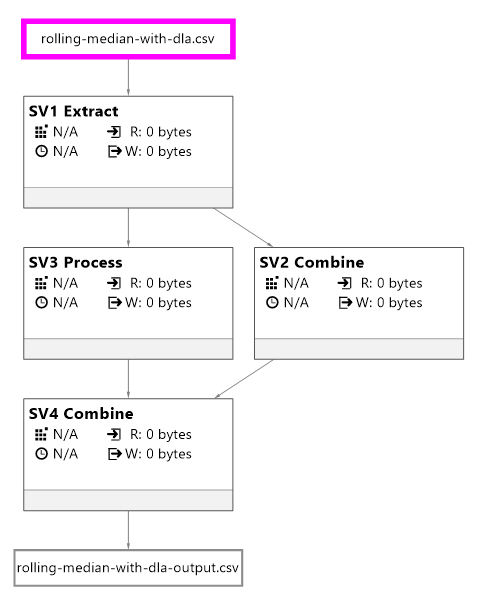
The file is then loaded into DLA with an EXTRACT statement. Note that we ensure that the time stamps are all UTC.
DECLARE @INPUT string = "rolling-median-with-dla.csv";
DECLARE @OUTPUT string = "rolling-median-with-dla-output.csv";
DECLARE @WINDOW_SIZE int = 11;


@Data =
    EXTRACT timestamp DateTime,
            site string,
            value1 double
    FROM @INPUT
    USING Extractors.Csv(quoting : true, skipFirstNRows : 1, silent : false);

// Adjust the timestamp to UTC
@Data =
    SELECT timestamp.ToUniversalTime() AS timestamp,
           site,
           value1
    FROM @Data;
This statement outlines how the rolling average will be calculated. Note that the window is centered and should be a odd number (11 in our case). Odd numbers are easier to deal with especially with the median later on.
@AvgData =
    SELECT timestamp,
           site,
           value1,

           AVG(value1) OVER(PARTITION BY site ORDER BY timestamp ROWS BETWEEN (@WINDOW_SIZE - 1) / 2 PRECEDING AND (@WINDOW_SIZE - 1) / 2 FOLLOWING) AS rolling_avg
    FROM @Data;
This is the key piece of code. We are performing a self-join. For each of the current record in the c table, we are joining the windowed records (in table w) by restricting the window through the BETWEEN operator.
Note the use of the DISTINCT operator as the PERCENTILE functions do not group the rows.
The continuous and discrete operators are used; more on that later.
@MedianData =
    SELECT DISTINCT c.timestamp,
           c.site,
           COUNT(*) OVER(PARTITION BY c.site, c.timestamp) AS row_count, // should be @WINDOW_SIZE * 2  + 1
           PERCENTILE_DISC(0.5) WITHIN GROUP(ORDER BY w.value1) OVER(PARTITION BY c.site, c.timestamp) AS rolling_median_disc,
           PERCENTILE_CONT(0.5) WITHIN GROUP(ORDER BY w.value1) OVER(PARTITION BY c.site, c.timestamp) AS rolling_median_cont
    FROM @Data AS c // current table
         INNER JOIN
             @Data AS w // windows table
         ON w.site == c.site
    WHERE w.timestamp BETWEEN c.timestamp.AddMinutes(-5 * (@WINDOW_SIZE - 1) / 2) AND c.timestamp.AddMinutes(5 * (@WINDOW_SIZE - 1) / 2)
   ;
The OUTPUT statement just save the results. Let’s analyse them.
OUTPUT
(
    SELECT a.timestamp, a.site, a.value1, a.rolling_avg, m.rolling_median_disc, m.rolling_median_cont
    FROM @AvgData AS a
    INNER JOIN @MedianData AS m ON m.timestamp == a.timestamp AND m.site == a.site
    ORDER BY site, timestamp
    OFFSET 0 ROWS
)
TO @OUTPUT
USING Outputters.Csv( outputHeader : true, dateTimeFormat : "u");
Reconciliation with R
The script is executed locally (it is a nice feature of DLA as it speed up the development of scripts as opposed as running the script from Azure). The output file can be found here.
Let’s make sure that the results are consistent with what we would have found with other means. For example, in R, the rollapply function with the partial parameter set to TRUE replicate the behavior of DLA. If partial is set to FALSE without padding (see na.pad), the first rows of each group will be removed as the data does not fit the window.
window_size = 11 # window size should be odd (for the rollmedian)

d.r = d %>%
  group_by(site) %>%
  mutate(
    rolling_avg = zoo::rollapply(data = value1, FUN = mean, align = "center", width = window_size, partial = T),
    rolling_median = zoo::rollapply(data = value1, align = "center", FUN = median, width = window_size, partial = T)
  )
A quick reconciliation with DLA (represented by the data frame d.dla) indicate that the values are similar.
reconciliation = d.r %>%
  rename(
    rolling_avg_r = rolling_avg,
    rolling_median_r = rolling_median
  ) %>%
  full_join(d.dla %>%
              rename(
                rolling_avg_dla = rolling_avg,
                rolling_median_cont_dla = rolling_median_cont,
                rolling_median_disc_dla = rolling_median_disc
              ), by = c("timestamp", "site", "value1")) %>%
  ungroup()

nrow(reconciliation %>%
  filter(
#    rolling_avg_r != rolling_avg_dla  |
    rolling_median_r != rolling_median_cont_dla
  ))
## [1] 0Note
There are differences between the rolling average in R and in DLA for the last 5 records of each group. I have not figured out why yet; I will submit the issue on stackoverflow.
PERCENTILE_DISC vs PERCENTILE_CONT
It is worth noting that PERCENTILE_DISC (the discrete implementation of the median) is different with the PERCENTILE_CONT for the first 5 rows of each group.
reconciliation %>%
  filter(site == "site1") %>%
  select(timestamp, value1, rolling_median_r, rolling_median_cont_dla, rolling_median_disc_dla)
## # A tibble: 100 x 5
## timestamp value1 rolling_median_r
## <dttm> <dbl> <dbl>
## 1 2017-01-01 00:00:00 0.3321 56.26
## 2 2017-01-01 00:05:00 95.6676 46.41
## 3 2017-01-01 00:10:00 74.8339 54.31
## 4 2017-01-01 00:15:00 46.4067 60.92
## 5 2017-01-01 00:20:00 66.1209 53.66
## 6 2017-01-01 00:25:00 4.9550 46.41
## 7 2017-01-01 00:30:00 26.3082 46.41
## 8 2017-01-01 00:35:00 62.2083 26.31
## 9 2017-01-01 00:40:00 60.9166 26.31
## 10 2017-01-01 00:45:00 16.3234 26.31
## # ... with 90 more rows, and 2 more variables:
## # rolling_median_cont_dla <dbl>, rolling_median_disc_dla <dbl>If we look at the first value with a centered window of size 11, only the current row and the next 5 rows will be taken into account. So, with the continuous median, the value is the middle between position 3 and 4 of the sorted values:
sorted_value = sort(reconciliation %>% filter(site == "site1") %>% head(6) %>% .$value1)
sorted_value
## [1] 0.3321 4.9550 46.4067 66.1209 74.8339 95.6676mean(sorted_value[3:4])## [1] 56.26With the discrete mean in ADL, it is the position 3 of the sorted vector.