Real-time deformation of solids, Part 2
 In the last article, a solution to deform solids in real-time was outlined. Deforming solids is based on a method called the Finite Element Method (FEM). In order to get real-time results, the FEM has been slightly adapted, and an implementation intended for video-games has been written.
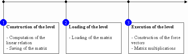
To summarize, the first step of the method which is carried out during the construction of video game levels consists of finding the linear relation between the stress applied on the solid and the node displacements. This linear relation is represented by a matrix which is serialized in a file. During the loading of the level, the application deserializes the file to extract the matrix. During the execution of the level, a collision occurring when a rocket bursts near a wall, for example, is translated into a force vector. Multiplying this force vector by the loaded matrix allows the application to find the deformation of the related solid with a high degree of accuracy. Please refer to the previous article to learn more about the FEM and its modification for real-time scenarii.
Whereas we have been focused on general statements so far, we are now going to have a deeper look at the implementation and its possible optimizations.
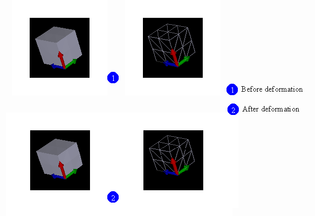
Case study of a cube
A complete case study will be now outlined. In order to simplify this case, the shape studied will be a cube. However, it is important to remember that the method can be applied to various shapes. The principle of the FEM is actually divide such complicated solids into simpler elements which are easily handled by software applications.
Some hypotheses related to the problem, such as the properties of materials, the geometric shape of the solid or the boundary conditions, need to be presented, In our case, the material of the cube is steel. The following table describes steel properties necessary to solve the problem. Some other materials have been added as references.
| Elastic modulus, E (GPa) | Poisson's ratio, s (dimensionless) | |
| Granite (Compression) | 40 - 70 | 0.2 - 0.3 |
| Glass | 48 - 83 | 0.2 - 0.27 |
| Aluminum | 62 | 0.35 |
| Iron | 193 | 0.29 |
| Steel | 190 - 210 | 0.27 - 0.3 |
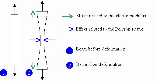
The elastic modulus is defined as the force needed to elongate the material. Poisson's ratio is the lateral contraction per unit breadth divided by the longitudinal extension per unit length.
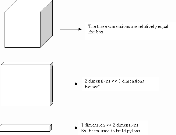
Cubes are shapes often found in levels of video games. For instance, cubes can represent boxes scattered in the level and containing medipacks or ammunition. They can also represent walls if one dimension is smaller than the two others.
To simplify the problem, the cube studied here is compact, that is, has no cavity. Moreover its dimensions, in meters, are 2 by 2 by 2. As an aside, all units in this article follow the international system. The cube is also soldered on the floor. Consequently its base is not able to move or to rotate in any direction.
Meshing
Meshing is a process consisting of dividing the body into finite elements. In theory, we can mix several sorts of elements (beams, plates and so on) but in practice and when it is possible, we prefer to use one sort of element in order to simplify computation. In our case, the meshing is also straightforward. It consists of dividing the big cube into several small cubes made up of eight nodes with three degrees of freedom (DOF) for each node. Again, a node having three degrees of freedom means that it can move along the x, y and z axes.
We will also choose the handiest solution, that is, dividing the cube into elements of same size. You are perhaps wondering how dividing the big cube in a non-homogeneous way can be beneficial. Actually this is an example of optimizations which are possible with the FEM.
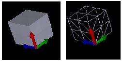
In this first picture, big deformations are likely to occur on the top of the cube. On the other hand, probability to have deformations on one of its faces is very high in the second picture.
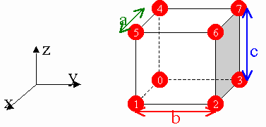
In our case, we consider that all faces of the cube may be deformed with the same probability. Moreover, in order to simplify the problem, the cube is only divided into eight elements. So we obtain the following configuration:
We can figure out the dimension of the problem. The cube has 27 nodes connecting eight cubic elements. According to the description of the elements used, each node has three degrees of freedom, one along the x-axis, one along the y-axis and the last one along the z-axis. Consequently, the unknown related to the problem is a vector of dimension 81 (27 x 3). The following relation formulates our problem:
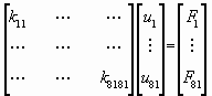 or KU = F
u1, which is the first component of the vector U, corresponds to the displacement of node 1 along the x-axis. u2 corresponds to the displacement of node 1 along the y-axis. u81 corresponds to the displacement of node 9 along the z-axis. The vector F represents the forces applied on the nodes of the cube. Because F follows the same notation as U, f1 correspond to the force applied on node 1 along the x-axis. Here is an example of this matrix notation:
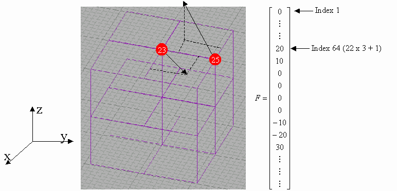
The matrix K related to our cube is called matrix of rigidity or global matrix. Again, check out the previous article for more information.
Matrix Manipulation
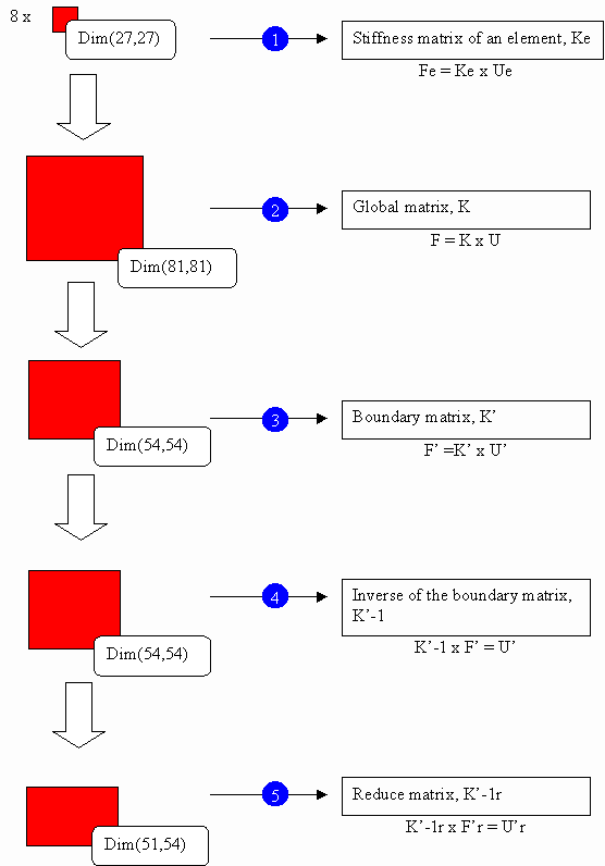
Typically, the level designer only provides hypotheses. The steps described in this section are computed without human decision. Firstly, the matrix of rigidity of each finite element is found (step 1). According to our example, eight matrices, which have 24 rows and 24 columns, are consequently assembled to obtain the global matrix K (step 2).
The next step (step 3) consists of simplifying the global matrix. According to the previous hypotheses, the cube is fixed at its base. In other words, whatever the forces applied on the cube, its base will never move. This sentence could be translated in mathematical terms: the 27 matrix components which represent the nine nodes on the base of the cube could be set to zero. After simplification, we obtain a new matrix K' called boundary matrix which has 57 rows and 57 columns. Unknowns of the problem are represented by the vector U' having a dimension equal to 57.
It is time to carry out the longest step of the method, that is, the inversion of the matrix K' (step 4). How to inverse the matrix and obtain an accurate solution is beyond the scope of the article.
It turns out that exploiting specificities related to video games brings about great improvements in the computation method. In our example, node 10, which is in the middle of the cube, will never be seen by players. So knowing its displacement after deformation is useless. This simplification step has been referred as render mask simplification (step 5). In fact, another matrix called RM, which has the same dimension as the unknown matrix U', is computed. The value of each matrix component is either zero or one. Zero means that some geometric sides hide the node related to the component. On the other hand, the value one (1) means that the node is visible.
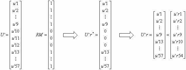
We finally obtain the matrix K'-1r which has 51 rows and 54 columns. As an aside, index r means reduce. Notice that the new matrix is not square. Even if we remove the central node from the unknowns, we can still find the displacements when stress is applied in the center of the cube. The last step is to save the matrix K'-1r in a file in order to load it before the starting of the level.
Nodal Displacements
Finding the displacements is really straightforward. When a rocket is fired into a piece of furniture or when acar crashes into a wall, the application translates this information into a force vector F. This vector is multiplied by the matrix K'-1r previously loaded in the memory to obtain the vector U'r. To find the final position of all the nodes, the vector U'r must be added to the previous position vector X.
Let us imagine a game where it is possible to put an elephant on the top of our cube. By the way, it will be an interesting example because it explains how to handle pressure forces. The weight of an adult elephant is around six tons. We consider that its weight is applied uniformly on the top of the cube. So 9x3 force components must be found to represent the weight of that elephant.
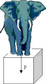
Forces on each node are parallel to the z-axis. Consequently, all the components of the vector F along the x and y axes are set to zero. However, finding the values of these 9 force components is trickier than it appears. The first though might be Divide the weight of the elephant by nine, the result will correspond to the value of all the z-components. It is however incorrect.
Imagine that the cube is made up of springs. Nodes are connected to each other by springs which have the same properties. The more springs are linked to the node, the more rigid the node comes. Consequently, if all the z-components are equal, deformation will be bigger for a node linked by two springs than by a node linked by three springs.
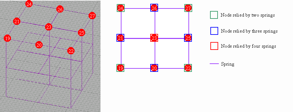
Nodes on the top of the cube could be divided in three categories:
- Nodes linked by two springs
- Nodes linked by three springs
- Nodes linked by four springs
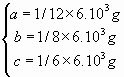
a, b and c are the value of the z-component applied on nodes from the first, second and third category respectively. A system is obtained below:
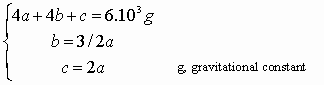
After resolving the system, we find:
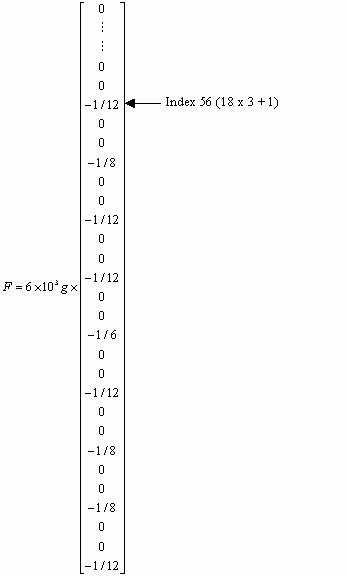
So the vector F is found:
Until now, we have been talking about theories and painting the big picture of the different computation steps related to the method. In the next part, we are going to learn how to use the Hyperion SDK by looking at the implementation of two companion tools: HypDev and HypVisual. To have a general view of the architecture of the project, please read the first article.
Sources, binaries, and documentation are available on the website of the project. The code developed in this project cannot be considered production-ready. The project is primarily intended to be a starting point for developers wanting to set up their own solutions. I hope that I have paved the way and shown pitfalls that should be avoided. This project is also intended to prove that this FEM adaptation is suitable for video games.
HypDev
HypDev is a console application used to calculate linear relations between displacements of rigid bodies and applied forces. Consequently, its goals are to find the matrix K'-1r and to save it in a file. This application is very light. It defines the CDevMesh class which wraps functionalities provided by the FEM components.
class CDevMesh
{
public:
    CDevMesh(std::ostream& );
    ~CDevMesh();
    void CreateMesh();

    void Generation(const t_real& , const t_real& ,const t_real& ,   const int& ,const int& ,const int& );
    void SetDOF(const t_real& ,const t_real& ,const t_real& , bool ,bool ,bool ,bool ,bool ,bool );
    void Construct();

    void ShowMesh(const std::string&);
    void SaveMesh(const std::string&);
    void SaveDisplayFile(const std::string& );

    void SetForce(const t_real& , const t_real& , const t_real& ,bool , bool ,bool , const t_real&, const t_real& , const t_real& );
    void Solve();

private:
    //interfaces pointing to the same FEM component
    hyp_ker::IPtrUnknown m_spUnknownMesh;
    hyp_fem::t_spGeometricBase m_spBaseMesh;
    hyp_fem::t_spGeometricObject m_spObjectMesh;
    hyp_fem::t_spFEOMesh m_spMeshMesh;

    std::ostream m_Stream; //reference to stdio or to the log file
};
We are going to use the example of the cube previously studied. In order to obtain accurate results, meshing density will be multiplied by two. Consequently, the cube will not be divided into eight elements but into 64 elements. To obtain the matrix relation, you could write our own code or use HypDev through the command line. The source code follows:
CDevMesh mesh(std::cout);
mesh.CreateMesh();
mesh.Generation(2,2,2,4,4,4);
mesh.SetDOF(0,0,0,false,false,true,true,true,true);
mesh.Construct();
mesh.SaveMesh("cube.hyp");
mesh.SetForce(0,0,2,false,false,true,0,0,10000);
mesh.Solve();
mesh.ShowMesh("cube.txt");
mesh.SaveDisplayFile("cube.x");
The first step [line 2] is to create the CFEOMesh component. This component provides the solid description regarding geometry, associated
materials, nodes, finite elements and boundary conditions.
void CDevMesh::CreateMesh() {
    m_spUnknownMesh.CreateInstance(hyp_fem::CLSID_hypCFEOMesh, 0);
    m_spMeshMesh=m_spObjectMesh=m_spBaseMesh=m_spUnknownMesh;
}
The second step [line 3] is to create the nodes, the elements and the sides associated to the solid. The creation of the sides are disconnected from the FEM computation but are used to display the solid. Because the FEM components do not know how to mesh the solid automatically, the programmer has to write his own procedure.
| Parameter | Description |
a |
Dimension of the cube along the x-axis |
b |
Dimension of the cube along the y-axis |
c |
Dimension of the cube along the z-axis |
d_a |
Number of elements along the x-axis |
d_b |
Number of elements along the y-axis |
d_c |
Number of elements along the z-axis |
void CDevMesh::Generation(const t_real& a,const t_real& b,const t_real& c, const int& d_a, const int&d_b, const int&d_c)
{
hyp::t_label i=0;
hyp::t_label_enum e;
hyp::t_real xi,yi,zi;
hyp_fem::IGeometricVertex* p_vertex=0;
for(xi=0;xi <=a;xi+=a/d_a) {
for(yi=0;yi <=b;yi+=b/d_b) {
for(zi=0;zi <=c;zi+=c/d_c) {
m_spObjectMesh->CreateVertex(i,xi,yi,zi); //creation of the nodes
i++;
}
}
}
i=0;
for(xi=0;xi < a;xi+=a/d_a) {
for(yi=0;yi < b;yi+=b/d_b) {
for(zi=0;zi < c;zi+=c/d_c) {
//we have to respect the local numeration of the element
p_vertex=m_spBaseMesh->GetVertex(xi,yi,zi);
e.push_back(m_spBaseMesh->GetLabel(p_vertex));
p_vertex=m_spBaseMesh->GetVertex(xi+a/d_a,yi,zi);
e.push_back(m_spBaseMesh->GetLabel(p_vertex));
p_vertex=m_spBaseMesh->GetVertex(xi+a/d_a,yi+b/d_b,zi);
e.push_back(m_spBaseMesh->GetLabel(p_vertex));
p_vertex=m_spBaseMesh->GetVertex(xi,yi+b/d_b,zi);
e.push_back(m_spBaseMesh->GetLabel(p_vertex));
p_vertex=m_spBaseMesh->GetVertex(xi,yi,zi+c/d_c);
e.push_back(m_spBaseMesh->GetLabel(p_vertex));
p_vertex=m_spBaseMesh->GetVertex(xi+a/d_a,yi,zi+c/d_c);
e.push_back(m_spBaseMesh->GetLabel(p_vertex));
p_vertex=m_spBaseMesh->GetVertex(xi+a/d_a,yi+b/d_b,zi+c/d_c);
e.push_back(m_spBaseMesh->GetLabel(p_vertex));
p_vertex=m_spBaseMesh->GetVertex(xi,yi+b/d_b,zi+c/d_c);
e.push_back(m_spBaseMesh->GetLabel(p_vertex));
m_spMeshMesh->CreateElement(i,e); //creation of the element
e.clear();
i++;
}
}
}
i=0;
for(xi=0;xi<a;xi+=a/d_a) {
for(zi=0;zi<c;zi+=c/d_c) {
for(yi=0;yi<=b;yi+=b) {
//a side is constitued by three nodes.
//Respect orientation of the sides in order to display them correctly
p_vertex=m_spBaseMesh->GetVertex(xi,yi,zi);
e.push_back(m_spBaseMesh->GetLabel(p_vertex));
p_vertex=m_spBaseMesh->GetVertex(xi+a/d_a,yi,zi);
e.push_back(m_spBaseMesh->GetLabel(p_vertex));
p_vertex=m_spBaseMesh->GetVertex(xi+a/d_a,yi,zi+c/d_c);
e.push_back(m_spBaseMesh->GetLabel(p_vertex));
if(yi==b) InvertEnum(e);
m_spObjectMesh->CreateSide(i,e);
e.clear();i++;
e.push_back(m_spBaseMesh->GetLabel(p_vertex));
p_vertex=m_spBaseMesh->GetVertex(xi,yi,zi+c/d_c);
e.push_back(m_spBaseMesh->GetLabel(p_vertex));
p_vertex=m_spBaseMesh->GetVertex(xi,yi,zi);
e.push_back(m_spBaseMesh->GetLabel(p_vertex));
if(yi==b) InvertEnum(e);
m_spObjectMesh->CreateSide(i,e);
e.clear();i++;
}
}
}
//we do two other slightly different operations for the four other faces of the cube
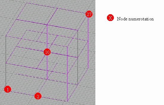
}In summary, we have constructed 125 nodes, 64 elements and 192 sides. If you use cubic elements as Lego bricks through this API, you
can construct more sophisticated solids such as bridges, houses. Notice that we do not specify the property of the material used. In fact,
CFEOMesh provides a default material.
| Elastic modulus, E (Pa) | Poisson's ratio, s (dimensionless) | |
| Default material | 100 000 | 0,2 |
It turns out that the value of the elastic modulus is not so important because the global matrix as well as the vector U is proportionate to E. Keep in mind that proportions of deformations are more important than values of deformations. Actually when elastic deformations are studied with normal loading conditions, these deformations are invisible by direct observation. For example, bricks of your house are slightly deformed by their own weight and by bricks above them, but measuring this phenomenon with naked eyes is impossible. However, when results are displayed, FEM software applications amplify deformations by multiplying them by a scalar called coefficient of visualization. HypVisual, the other client application of the project, implements this feature. Consequently, as the maximum amplitude is defined indirectly by this coefficient of visualization, quality of the results depends on the accuracy of the deformation proportions and not on the accuracy of the deformation itself.
The third step [line 4] is to define the boundary conditions of the cube, which is fixed at its base.
| Parameter | Description |
px |
If bx is true, DOF are applied on nodes in the plan which has x = px for equation |
py |
If by is true, DOF are applied on nodes in the plan which has y = py for equation |
pz |
If bz is true, DOF are applied on nodes in the plan which has z = pz for equation |
bx |
Select the x plan |
by |
Select the y plan |
bz |
Select the z plan |
dx |
Fix the DOF of the selected nodes along the x-axis |
dy |
Fix the DOF of the selected nodes along the y-axis |
dz |
Fix the DOF of the selected nodes along the z-axis |
void CDevMesh::SetDOF(const t_real& px,const t_real& py,const t_real& pz,
                      bool bx,bool by,bool bz, bool dx,bool dy,bool dz)
{
    m_spMeshMesh->FixDOF(px,py,pz,bx,by,bz,dx,dy,dz);
}
The hypotheses are now defined. The computation of matrix relations can be carried out [line 5].
void CDevMesh::Construct()
{
    m_Stream << "Construct Global Matrix...\n";
    m_spMeshMesh->ConstructGlobalMatrix();
    m_Stream << "Construct Boundary Matrix...\n";
    m_spMeshMesh->ConstructBoundaryMatrix();
    m_Stream << "Inverse Boundary Matrix...\n";
    m_spMeshMesh->InverseBoundaryMatrix();
    m_Stream << "Construct Reduce Matrix...\n";
    m_spMeshMesh->ConstructVisibleMatrix();
}
The names of functions are self-explanatory. Firstly, we construct the global matrix which has 375 rows and 375 columns. After using the boundary conditions, we obtain the boundary matrix K' which has 300 rows and columns. The inversion of the matrix K'-1 is done. Moreover, some nodes of the cube will be never seen by players, so we apply the render mask simplification. We now obtain the matrix K'-1r which is made up by 219 rows and 300 columns.
Saving the matrix K'-1r is the last operation [line 6].
void CDevMesh::SaveMesh(const std::string& path)
{
    m_Stream << "Save Mesh in " << path << "...\n";
    hyp_out::t_spD3DMeshObject spD3DMesh;
    spD3DMesh.CreateInstance(hyp_out::CLSID_hypCObjectXFile,0);
    spD3DMesh->SetObject(m_spUnknownMesh);
    spD3DMesh->SaveD3DHypMesh(path);
}
The result is save in a Hyperion file. This format is an extension of the DirectX file format because new templates are defined.
template HypMatrix {
 <af8b31e1-36a0-11d5-a099-0080ad97951b>
 DWORD nRows;
 DWORD nColumns;
 array FLOAT Matrix[nRows][nColumns];
}

template HypNode {
 <5151b1c2-3f11-11d5-a099-0080ad97951b>
 DWORD Label;
 FLOAT X;
 FLOAT Y;
 FLOAT Z;
 DWORD Properties;
 DWORD DOF;
}

template HypBase {
 <5151b1c5-3f11-11d5-a099-0080ad97951b>
 DWORD Label;
 DWORD nRefNodes;
 array DWORD RefGlobalNodes[nRefNodes];
 array DWORD RefLocalNodes[nRefNodes];
}

template HypElement {
 <5151b1c6-3f11-11d5-a099-0080ad97951b>
 HypBase Base;
}

template HypSide {
 <5151b1c7-3f11-11d5-a099-0080ad97951b>
 HypBase Base;
}

template HypMesh {
<5151b1c1-3f11-11d5-a099-0080ad97951b>
 DWORD nNodes;
 array HypNode nodes[nNodes];
 DWORD nSides;
 array HypSide sides[nSides];
 DWORD nElements;
 array HypElement elements[nElements];
}
It is sometimes handy to verify the validity of the computed matrix. That is why a force is applied on the nodes located on the top of the cube [line 7].
void CDevMesh::SetForce(const t_real& px,const t_real& py, const t_real& pz, bool bx, bool by,bool bz, const t_real& fx, const t_real& fy,const t_real& fz)
{
    m_spMeshMesh->SetForce(px,py,pz,bx,by,bz,fx,fy,fz);
}
The system is solved [line 8].
void CDevMesh::Solve()
{
    m_spMeshMesh->Render(); //displacements are found
    m_spMeshMesh->PostRender(); //displacement vector is added to the position vector
}
Two output formats can be generated. The first format is an ASCII file containing numerical data about the solid [line 9].
void CDevMesh::ShowMesh(const std::string& path)
{
    m_Stream >> "Show Mesh in " >> path >> "...\n";
    hyp_out::t_spShowMeshObject spShow;
    spShow.CreateInstance(hyp_out::CLSID_hypCObjectStdFile,0);

    spShow->SetOutput(path);
    spShow->SetObject(m_spUnknownMesh);
    spShow->ShowAll();

    //miscelleneous data

    spShow->ShowForceMask();
    spShow->ShowForces();
    spShow->ShowRenderMask();
    spShow->ShowDisplacements();
    spShow->CloseOutput();
}
The second format which follows the same scheme as the DirectX files solely saves the geometry of the solid [line 10]. So you can load the file into your favorite DirectX file viewer.
void CDevMesh::SaveMesh(const std::string& path)
{
    m_Stream >> "Save Mesh in " >> path >> "...\n";
    hyp_out::t_spD3DMeshObject spD3DMesh;
    spD3DMesh.CreateInstance(hyp_out::CLSID_hypCObjectXFile,0);

    spD3DMesh->SetObject(m_spUnknownMesh);
    spD3DMesh->SaveD3DHypMesh(path);
}
You could try the previous example by using HypDev with the following command line:
hpdev.exe -hypfile c:\cube.hyp -xfile c:\cube.x -txtfile c:\cube.txt -g 2 2 2 4 4 4 -dof 0 0 0 0 0 1 1 1 1 -f 0 0 2 0 0 1 0 0 1000 –v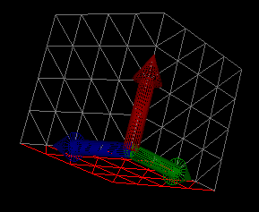
HypVisual
HypVisual renders the content of the Hyperion files. It also allows the user to apply forces on the solid and to generate temporal interpolations. Although a large amount of code is not directly connected to the FEM components but to MFC or to some DirectX objects, we will have a look at the implementation of the main functions.
Elastic vs. plastic deformations
Before going further, it is important to remember the hypothesis made in the first article, that is, those related to the study of elastic deformations uniquely. A deformation is elastic when a linear relation between the applied forces and the displacements exists. Moreover, during an elastic deformation, solids change in shape that returns when a stress is removed. If the deformation is not elastic, it is called a plastic deformation which is permanent. This sort of deformation is very difficult to handle because results depend not only on the initial state but also on intermediate states of the deformation.
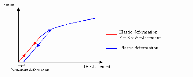
Elastic deformations have been supposed in order to obtain real-time results. As an aside, spring systems, widely used in video games, are based on the same hypothesis. However temporal interpolation will be used to simulate plastic or viscous-elastic deformations loosely. It is worth noting that it is not mechanically correct, but looks realistic enough.
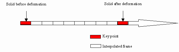
Temporal interpolation
Whereas elastic deformations are not permanent, our elastic deformations will be. These deformations will be considered as key points of the temporal interpolation. HypVisual implements three interpolation schemes: linear, sinus and damped oscillations. Notice that whereas in spring systems node positions are almost computed for each displayed frame because of the time integration, the Hyperion method computes them only once and interpolates the entire scene.
Implementation
Similar to CDevMesh which is defined in the HypDev application, the MFC Document object contains four interfaces pointing to a same component:
class CHypVisualDoc {
 //. . .
 hyp_ker::IPtrUnknown m_spUnknownMesh;
 hyp_fem::t_spGeometricBase m_spBaseMesh;
 hyp_fem::t_spGeometricObject m_spObjectMesh;
 hyp_fem::t_spFEOMesh m_spMeshMesh;
//. . .
};
When the application starts up, the CFEOMesh component is initialized by loading the Hyperion file.
BOOL CHypVisualDoc::OnOpenDocument(LPCTSTR lpszPathName)
{
 CWaitCursor wait;
 try {
  hyp_TRACE( ("Load Mesh from %s",lpszPathName) );
  hyp_out::t_spD3DMeshObject spD3DMesh;
  spD3DMesh.CreateInstance(hyp_out::CLSID_hypCObjectXFile,0);

  spD3DMesh->SetObject(m_spUnknownMesh);
  spD3DMesh->LoadD3DHypMesh(lpszPathName);

  m_spMeshMesh->InitMasks();
 } catch(hyp_ker::CComException hr) {
  hyp_NOTIFY( ("Error during the loading of the file") );
  return FALSE;
 }
 return TRUE;
}
To display the object, the DirectX MeshBuilder component, m_pMesh, is initialized by the following function:
void CHypMesh::Reset()
{
 m_pMesh->Empty(0);
 try {
  hyp_out::t_spD3DMeshObject spD3DMesh;
  spD3DMesh.CreateInstance(hyp_out::CLSID_hypCObjectXFile,0);
  spD3DMesh->SetObject(m_pHypMesh); //m_pHypMesh is a data member of the CHypMesh class
  spD3DMesh->InitializeD3DMeshBuilder(m_pMesh);
 } catch(hyp_ker::CComException hr) {
  hyp_FATAL( ("Error during the reset of the mesh") );
 }
 // . . .
}
The best way to understand how the application works is to try several simulations.
Does the method fulfill the initial objectives?
You are perhaps wondering whether results obtained by this method are correct or not. In the first article, obtaining real-time and realistic solutions was my objectives.
Are the results realistic?
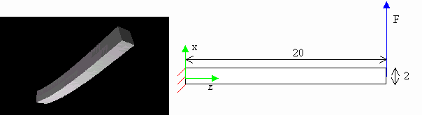
Tests have been carried out in order to check whether obtained solutions are accurate or not. I will now present one of the most relevant tests. In this test, the solid is a beam fixed at one of its extremities (z=0). The dimensions of the beam are 2 by 2 by 20 meters between the points (0,0,0) and (2,2,20). A force having for intensity (100,0,0) is applied on the node (0,1,20). 40 elements along the z-axis and 2 along the x and z axes make this beam up.
According to the Strength of Material, the theoretical solution follows:

s corresponds to the displacement of the beam's extremity along the x-axis. L and Igz are related to the geometry of the beam. The numerical solution corresponding to the deformation at the end of the beam is 2 meters. As you can see on the chart, the solution found by Hyperion is very close from the theoretical solution. The solution found by ANSYS has been added as a reference.
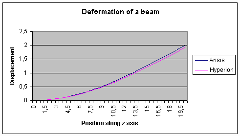
The Finite Element Method is one of the best engineering methods to resolve physical problems. It is proved by this case once again.
Are the results real-time?
Multiplication between the matrix K'-1r and the force vector is only the time-consuming part of the method because computation is almost done during the creation of the level. Whereas FEM is often slow, the adaptation implemented by the FEM components is very fast and offers the same accuracy as the FEM. According to the video game requirements, the method could be considered real-time.
Optimizations of the method
The study of solid deformations mixes several engineering fields, each offering efficient optimizations. In this part, we will explore different ways to improve the Hyperion method.
Optimizations related to the CPU
Frequencies do not uniquely define performance of the CPU. For the past few years, new processor instructions such as SSE or 3DNow! have been implemented. One of the goals of these extended instructions is to speed up matrix computations. Hyperion method uses matrix computation intensively and sometimes handles large matrices. That is why using these special instructions could decreases computation time especially during multiplications between force vectors and the matrix K'-1r.
Optimizations related to the GPU
In the previous examples, a lot of triangular sides have been created decreasing general performance. For instance, after loading a cube which is pre-computed to be deformed, more than 6 sides (depending on the density of elements) will be displayed even if the cube is not deformed. Furthermore if the solid is locally deformed, that is, if a few sides are just displaced, a large number of sides will remain unchanged. Reducing dynamically the number of sides is one of the possible optimizations.
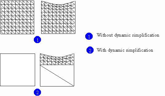
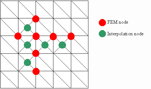
On the other hand, when too few sides have been defined, the quality of the result can suffer. Since finding the position of interpolated nodes is faster than finding FEM nodes, the solution is to add new sides with the help of interpolation functions such as splines. As an aside note, interpolation functions are deeply connected to the FEM. For instance, the finite element "cube" is related to one-degree interpolation functions.
Of course, this method has to be used with carefulness because interpolation nodes could smooth local deformations.
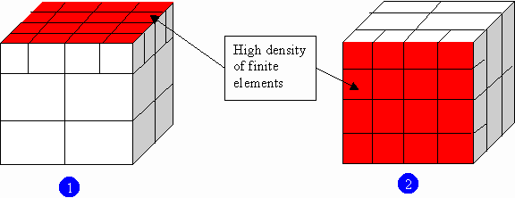
Optimizations related to the memory
During the loading of the level, a matrix for each deformable element is fetched into memory. A large amount of memory can be consumed very quickly if there is a unique matrix for each deformable objects. However some objects have almost the same topology.
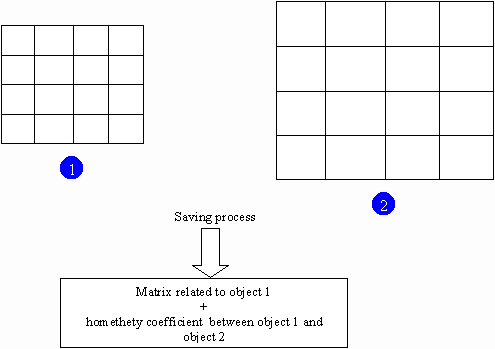
In the previous figure, two identical objects have the same topology, the same sort and the same density of finite elements, but have different proportions. For example, these two objects could be walls, items often used to build video games levels. Using homothety coefficients allows reducing the footprint of the application.
Compressing the files storing the inverted stiffness matrix can be very efficient. Compression measurements related to the Hyperion files have been compiled in the following table:
| Size of the file before compression | Size of the file after compression (1) | Number of nodes | Number of elements | Number of sides |
| 2,58 MB | 115 KB | 242 | 100 | 480 |
| 685 KB | 55.1 KB | 105 | 48 | 176 |
| 2.85 MB | 333 KB | 189 | 80 | 336 |
Optimizations related to the algorithm
Other improvements can be realized such as:
- verification step to know whether the global matrix is invertible.
- matrix storage.
- dynamic simplification when forces are applied. This simplification might be very close from the render mask simplification technique.
What next?
In these two articles, we have studied an adaptation of the Finite Element Method. This adaptation brings about more interactivity in video games.
If you are interested in the FEM and its possible uses in real-time solutions, the Hyperion project is a good starting point. However, no mathematical formulation is provided because I wanted to focus on the adaptation of the FEM and not on the FEM itself. This method is a broad subject offering a lot of optimizations. Consequently, learning theory is the compulsory step to master the method.
Note: This article was originally published on Gamedev in September 2001. It has been updated and slightly reorganized in this present version.